23. Heterogeneous Beliefs and Financial Markets#
23.1. Overview#
A likelihood ratio process lies behind Lawrence Blume and David Easley’s answer to their question ‘‘If you’re so smart, why aren’t you rich?’’ [Blume and Easley, 2006].
Blume and Easley constructed formal models to study how differences of opinions about probabilities governing risky income processes would influence outcomes and be reflected in prices of stocks, bonds, and insurance policies that individuals use to share and hedge risks.
Note
[Alchian, 1950] and [Friedman, 1953] conjectured that, by rewarding traders with more realistic probability models, competitive markets in financial securities put wealth in the hands of better informed traders and help make prices of risky assets reflect realistic probability assessments.
Here we’ll provide an example that illustrates basic components of Blume and Easley’s analysis.
We’ll focus only on their analysis of an environment with complete markets in which trades in all conceivable risky securities are possible.
We’ll study two alternative arrangements:
perfect socialism in which individuals surrender their endowments of consumption goods each period to a central planner who then dictatorially allocates those goods
a decentralized system of competitive markets in which selfish price-taking individuals voluntarily trade with each other in competitive markets
The fundamental theorems of welfare economics will apply and assure us that these two arrangements end up producing exactly the same allocation of consumption goods to individuals provided that the social planner assigns an appropriate set of Pareto weights.
Note
You can learn about how the two welfare theorems are applied in modern macroeconomic models in this lecture on a planning problem and this lecture on a related competitive equilibrium. This quantecon lecture presents a recursive formulation of complete markets models with homogeneous beliefs.
Let’s start by importing some Python tools.
import matplotlib.pyplot as plt
import numpy as np
from numba import vectorize, jit, prange
from math import gamma
from scipy.integrate import quad
23.2. Review: likelihood ratio processes#
We’ll begin by reminding ourselves definitions and properties of likelihood ratio processes.
A nonnegative random variable \(W\) has one of two probability density functions, either \(f\) or \(g\).
Before the beginning of time, nature once and for all decides whether she will draw a sequence of IID draws from either \(f\) or \(g\).
We will sometimes let \(q\) be the density that nature chose once and for all, so that \(q\) is either \(f\) or \(g\), permanently.
Nature knows which density it permanently draws from, but we the observers do not.
We know both \(f\) and \(g\) but we don’t know which density nature chose.
But we want to know.
To do that, we use observations.
We observe a sequence \(\{w_t\}_{t=1}^T\) of \(T\) IID draws that we know came from either \(f\) or \(g\).
We want to use these observations to infer whether nature chose \(f\) or \(g\).
A likelihood ratio process is a useful tool for this task.
To begin, we define a key component of a likelihood ratio process, namely, the time \(t\) likelihood ratio as the random variable
We assume that \(f\) and \(g\) both put positive probabilities on the same intervals of possible realizations of the random variable \(W\).
That means that under the \(g\) density, \(\ell (w_t)= \frac{f\left(w_{t}\right)}{g\left(w_{t}\right)}\) is a nonnegative random variable with mean \(1\).
A likelihood ratio process for sequence \(\left\{ w_{t}\right\} _{t=1}^{\infty}\) is defined as
where \(w^t=\{ w_1,\dots,w_t\}\) is a history of observations up to and including time \(t\).
Sometimes for shorthand we’ll write \(L_t = L(w^t)\).
Notice that the likelihood process satisfies the recursion
The likelihood ratio and its logarithm are key tools for making inferences using a classic frequentist approach due to Neyman and Pearson [Neyman and Pearson, 1933].
To help us appreciate how things work, the following Python code evaluates \(f\) and \(g\) as two different Beta distributions, then computes and simulates an associated likelihood ratio process by generating a sequence \(w^t\) from one of the two probability distributions, for example, a sequence of IID draws from \(g\).
# Parameters in the two Beta distributions.
F_a, F_b = 1, 1
G_a, G_b = 3, 1.2

@vectorize
def p(x, a, b):
    r = gamma(a + b) / (gamma(a) * gamma(b))
    return r * x** (a-1) * (1 - x) ** (b-1)

# The two density functions.
f = jit(lambda x: p(x, F_a, F_b))
g = jit(lambda x: p(x, G_a, G_b))
@jit
def simulate(a, b, T=50, N=500):
    '''
    Generate N sets of T observations of the likelihood ratio,
    return as N x T matrix.
    '''

    l_arr = np.empty((N, T))

    for i in range(N):
        for j in range(T):
            w = np.random.beta(a, b)
            l_arr[i, j] = f(w) / g(w)

    return l_arr
23.3. Blume and Easley’s setting#
Let the random variable \(s_t \in (0,1)\) at time \(t =0, 1, 2, \ldots\) be distributed according to the same Beta distribution with parameters \(\theta = \{\theta_1, \theta_2\}\).
We’ll denote this probability density as
Below, we’ll often just write \(\pi(s_t)\) instead of \(\pi(s_t|\theta)\) to save space.
Let \(s_t \equiv y_t^1\) be the endowment of a nonstorable consumption good that a person we’ll call “agent 1” receives at time \(t\).
Let a history \(s^t = [s_t, s_{t-1}, \ldots, s_0]\) be a sequence of i.i.d. random variables with joint distribution
So in our example, the history \(s^t\) is a comprehensive record of agent \(1\)’s endowments of the consumption good from time \(0\) up to time \(t\).
If agent \(1\) were to live on an island by himself, agent \(1\)’s consumption \(c^1(s_t)\) at time \(t\) is
But in our model, agent 1 is not alone.
23.4. Nature and agents’ beliefs#
Nature draws i.i.d. sequences \(\{s_t\}_{t=0}^\infty\) from \(\pi_t(s^t)\).
so \(\pi\) without a superscript is nature’s model
but in addition to nature, there are other entities inside our model – artificial people that we call “agents”
each agent has a sequence of probability distributions over \(s^t\) for \(t=0, \ldots\)
agent \(i\) thinks that nature draws i.i.d. sequences \(\{s_t\}_{t=0}^\infty\) from \(\{\pi_t^i(s^t)\}_{t=0}^\infty\)
agent \(i\) is mistaken unless \(\pi_t^i(s^t) = \pi_t(s^t)\)
Note
A rational expectations model would set \(\pi_t^i(s^t) = \pi_t(s^t)\) for all agents \(i\).
There are two agents named \(i=1\) and \(i=2\).
At time \(t\), agent \(1\) receives an endowment
of a nonstorable consumption good, while agent \(2\) receives an endowment of
The aggregate endowment of the consumption good is
at each date \(t \geq 0\).
At date \(t\) agent \(i\) consumes \(c_t^i(s^t)\) of the good.
A (non wasteful) feasible allocation of the aggregate endowment of \(1\) each period satisfies
23.7. If you’re so smart, \(\ldots\)#
Let’s compute some values of limiting allocations (23.5) for some interesting possible limiting values of the likelihood ratio process \(l_t(s^t)\):
In the above case, both agents are equally smart (or equally not smart) and the consumption allocation stays put at a \(\lambda, 1 - \lambda\) split between the two agents.
In the above case, agent 2 is ‘‘smarter’’ than agent 1, and agent 1’s share of the aggregate endowment converges to zero.
In the above case, agent 1 is smarter than agent 2, and agent 1’s share of the aggregate endowment converges to 1.
Note
These three cases are somehow telling us about how relative wealths of the agents evolve as time passes.
when the two agents are equally smart and \(\lambda \in (0,1)\), agent 1’s wealth share stays at \(\lambda\) perpetually.
when agent 1 is smarter and \(\lambda \in (0,1)\), agent 1 eventually “owns” the entire continuation endowment and agent 2 eventually “owns” nothing.
when agent 2 is smarter and \(\lambda \in (0,1)\), agent 2 eventually “owns” the entire continuation endowment and agent 1 eventually “owns” nothing. Continuation wealths can be defined precisely after we introduce a competitive equilibrium price system below.
Soon we’ll do some simulations that will shed further light on possible outcomes.
But before we do that, let’s take a detour and study some “shadow prices” for the social planning problem that can readily be converted to “equilibrium prices” for a competitive equilibrium.
Doing this will allow us to connect our analysis with an argument of [Alchian, 1950] and [Friedman, 1953] that competitive market processes can make prices of risky assets better reflect realistic probability assessments.
23.8. Competitive equilibrium prices#
Two fundamental welfare theorems for general equilibrium models lead us to anticipate that there is a connection between the allocation that solves the social planning problem we have been studying and the allocation in a competitive equilibrium with complete markets in history-contingent commodities.
Note
For the two welfare theorems and their history, see https://en.wikipedia.org/wiki/Fundamental_theorems_of_welfare_economics. Again, for applications to a classic macroeconomic growth model, see this lecture on a planning problem and this lecture on a related competitive equilibrium
Such a connection prevails for our model.
We’ll sketch it now.
In a competitive equilibrium, there is no social planner that dictatorially collects everybody’s endowments and then reallocates them.
Instead, there is a comprehensive centralized market that meets at one point in time.
There are prices at which price-taking agents can buy or sell whatever goods that they want.
Trade is multilateral in the sense that that there is a “Walrasian auctioneer” who lives outside the model and whose job is to verify that each agent’s budget constraint is satisfied.
That budget constraint involves the total value of the agent’s endowment stream and the total value of its consumption stream.
These values are computed at price vectors that the agents take as given – they are “price-takers” who assume that they can buy or sell whatever quantities that they want at those prices.
Suppose that at time \(-1\), before time \(0\) starts, agent \(i\) can purchase one unit \(c_t(s^t)\) of consumption at time \(t\) after history \(s^t\) at price \(p_t(s^t)\).
Notice that there is (very long) vector of prices.
there is one price \(p_t(s^t)\) for each history \(s^t\) at every date \(t = 0, 1, \ldots, \).
so there are as many prices as there are histories and dates.
These prices determined at time \(-1\) before the economy starts.
The market meets once at time \(-1\).
At times \(t =0, 1, 2, \ldots\) trades made at time \(-1\) are executed.
in the background, there is an “enforcement” procedure that forces agents to carry out the exchanges or “deliveries” that they agreed to at time \(-1\).
We want to study how agents’ beliefs influence equilibrium prices.
Agent \(i\) faces a single intertemporal budget constraint
According to budget constraint (23.6), trade is multilateral in the following sense
we can imagine that agent \(i\) first sells his random endowment stream \(\{y_t^i (s^t)\}\) and then uses the proceeds (i.e., his “wealth”) to purchase a random consumption stream \(\{c_t^i (s^t)\}\).
Agent \(i\) puts a Lagrange multiplier \(\mu_i\) on (23.6) and once-and-for-all chooses a consumption plan \(\{c^i_t(s^t)\}_{t=0}^\infty\) to maximize criterion (23.2) subject to budget constraint (23.6).
This means that the agent \(i\) chooses many objects, namely, \(c_t^i(s^t)\) for all \(s^t\) for \(t = 0, 1, 2, \ldots\).
For convenience, let’s remind ourselves of criterion \(V^i\) defined in (23.2):
First-order necessary conditions for maximizing objective \(V^i\) defined in (23.2) with respect to \(c_t^i(s^t)\) are
which we can rearrange to obtain
for \(i=1,2\).
If we divide equation (23.7) for agent \(1\) by the appropriate version of equation (23.7) for agent 2, use \(c^2_t(s^t) = 1 - c^1_t(s^t)\), and do some algebra, we’ll obtain
We now engage in an extended “guess-and-verify” exercise that involves matching objects in our competitive equilibrium with objects in our social planning problem.
we’ll match consumption allocations in the planning problem with equilibrium consumption allocations in the competitive equilibrium
we’ll match “shadow” prices in the planning problem with competitive equilibrium prices.
Notice that if we set \(\mu_1 = 1-\lambda\) and \(\mu_2 = \lambda\), then formula (23.8) agrees with formula (23.5).
doing this amounts to choosing a numeraire or normalization for the price system \(\{p_t(s^t)\}_{t=0}^\infty\)
Note
For information about how a numeraire must be chosen to pin down the absolute price level in a model like ours that determines only relative prices, see https://en.wikipedia.org/wiki/Numéraire.
If we substitute formula (23.8) for \(c_t^1(s^t)\) into formula (23.7) and rearrange, we obtain
or
According to formula (23.9), we have the following possible limiting cases:
when \(l_\infty = 0\), \(c_\infty^1 = 0 \) and tails of competitive equilibrium prices reflect agent \(2\)’s probability model \(\pi_t^2(s^t)\) according to \(p_t(s^t) \propto \delta^t \pi_t^2(s^t) \)
when \(l_\infty = \infty\), \(c_\infty^1 = 1 \) and tails of competitive equilibrium prices reflect agent \(1\)’s probability model \(\pi_t^1(s^t)\) according to \(p_t(s^t) \propto \delta^t \pi_t^1(s^t) \)
for small \(t\)’s, competitive equilibrium prices reflect both agents’ probability models.
We leave the verification of the shadow prices to the reader since it follows from the same reasoning.
23.9. Simulations#
Now let’s implement some simulations when agent \(1\) believes marginal density
and agent \(2\) believes marginal density
where \(f\) and \(g\) are Beta distributions like ones that we used in earlier sections of this lecture.
Meanwhile, we’ll assume that nature believes a marginal density
where \(h(s_t)\) is perhaps a mixture of \(f\) and \(g\).
First, we write a function to compute the likelihood ratio process
def compute_likelihood_ratios(sequences, f, g):
    """Compute likelihood ratios and cumulative products."""
    l_ratios = f(sequences) / g(sequences)
    L_cumulative = np.cumprod(l_ratios, axis=1)
    return l_ratios, L_cumulative
Let’s compute the Kullback–Leibler discrepancies by quadrature integration.
def compute_KL(f, g):
    """
    Compute KL divergence KL(f, g)
    """
    integrand = lambda w: f(w) * np.log(f(w) / g(w))
    val, _ = quad(integrand, 1e-5, 1-1e-5)
    return val
We also create a helper function to compute KL divergence with respect to a reference distribution \(h\)
def compute_KL_h(h, f, g):
    """
    Compute KL divergence with reference distribution h
    """

    Kf = compute_KL(h, f)
    Kg = compute_KL(h, g)

    return Kf, Kg
Let’s write a Python function that computes agent 1’s consumption share
def simulate_blume_easley(sequences, f_belief=f, g_belief=g, λ=0.5):
    """Simulate Blume-Easley model consumption shares."""
    l_ratios, l_cumulative = compute_likelihood_ratios(sequences, f_belief, g_belief)
    c1_share = λ * l_cumulative / (1 - λ + λ * l_cumulative)
    return l_cumulative, c1_share
Now let’s use this function to generate sequences in which
nature draws from \(f\) each period, or
nature draws from \(g\) each period, or
nature flips a fair coin each period to decide whether to draw from \(f\) or \(g\)
λ = 0.5
T = 100
N = 10000

# Nature follows f, g, or mixture
s_seq_f = np.random.beta(F_a, F_b, (N, T))
s_seq_g = np.random.beta(G_a, G_b, (N, T))

h = jit(lambda x: 0.5 * f(x) + 0.5 * g(x))
model_choices = np.random.rand(N, T) < 0.5
s_seq_h = np.empty((N, T))
s_seq_h[model_choices] = np.random.beta(F_a, F_b, size=model_choices.sum())
s_seq_h[~model_choices] = np.random.beta(G_a, G_b, size=(~model_choices).sum())

l_cum_f, c1_f = simulate_blume_easley(s_seq_f)
l_cum_g, c1_g = simulate_blume_easley(s_seq_g)
l_cum_h, c1_h = simulate_blume_easley(s_seq_h)
Before looking at the figure below, have some fun by guessing whether agent 1 or agent 2 will have a larger and larger consumption share as time passes in our three cases.
To make better guesses, let’s visualize instances of the likelihood ratio processes in the three cases.
fig, axes = plt.subplots(2, 3, figsize=(15, 10))

titles = ["Nature = f", "Nature = g", "Nature = mixture"]
data_pairs = [(l_cum_f, c1_f), (l_cum_g, c1_g), (l_cum_h, c1_h)]

for i, ((l_cum, c1), title) in enumerate(zip(data_pairs, titles)):
    # Likelihood ratios
    ax = axes[0, i]
    for j in range(min(50, l_cum.shape[0])):
        ax.plot(l_cum[j, :], alpha=0.3, color='blue')
    ax.set_yscale('log')
    ax.set_xlabel('time')
    ax.set_ylabel('Likelihood ratio $l_t$')
    ax.set_title(title)
    ax.axhline(y=1, color='red', linestyle='--', alpha=0.5)

    # Consumption shares
    ax = axes[1, i]
    for j in range(min(50, c1.shape[0])):
        ax.plot(c1[j, :], alpha=0.3, color='green')
    ax.set_xlabel('time')
    ax.set_ylabel("Agent 1's consumption share")
    ax.set_ylim([0, 1])
    ax.axhline(y=λ, color='red', linestyle='--', alpha=0.5)

plt.tight_layout()
plt.show()
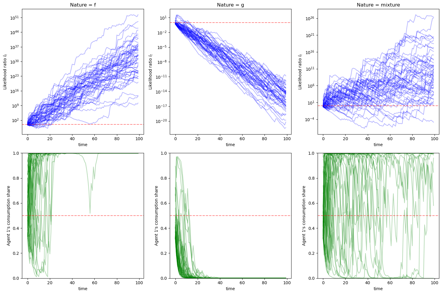
In the left panel, nature chooses \(f\). Agent 1’s consumption reaches \(1\) very quickly.
In the middle panel, nature chooses \(g\). Agent 1’s consumption ratio tends to move towards \(0\) but not as fast as in the first case.
In the right panel, nature flips coins each period. We see a very similar pattern to the processes in the left panel.
The figures in the top panel remind us of the discussion in this section.
We invite readers to revisit that section and try to infer the relationships among \(D_{KL}(f\|g)\), \(D_{KL}(g\|f)\), \(D_{KL}(h\|f)\), and \(D_{KL}(h\|g)\).
Let’s compute values of KL divergence
shares = [np.mean(c1_f[:, -1]), np.mean(c1_g[:, -1]), np.mean(c1_h[:, -1])]
Kf_g, Kg_f = compute_KL(f, g), compute_KL(g, f)
Kf_h, Kg_h = compute_KL_h(h, f, g)

print(f"Final shares: f={shares[0]:.3f}, g={shares[1]:.3f}, mix={shares[2]:.3f}")
print(f"KL divergences: \nKL(f,g)={Kf_g:.3f}, KL(g,f)={Kg_f:.3f}")
print(f"KL(h,f)={Kf_h:.3f}, KL(h,g)={Kg_h:.3f}")
Final shares: f=1.000, g=0.000, mix=0.921
KL divergences:
KL(f,g)=0.759, KL(g,f)=0.344
KL(h,f)=0.073, KL(h,g)=0.281
We find that \(KL(f,g) > KL(g,f)\) and \(KL(h,g) > KL(h,f)\).
The first inequality tells us that the average “surprise” from having belief \(g\) when nature chooses \(f\) is greater than the “surprise” from having belief \(f\) when nature chooses \(g\).
This explains the difference between the first two panels we noted above.
The second inequality tells us that agent 1’s belief distribution \(f\) is closer to nature’s pick than agent 2’s belief \(g\).
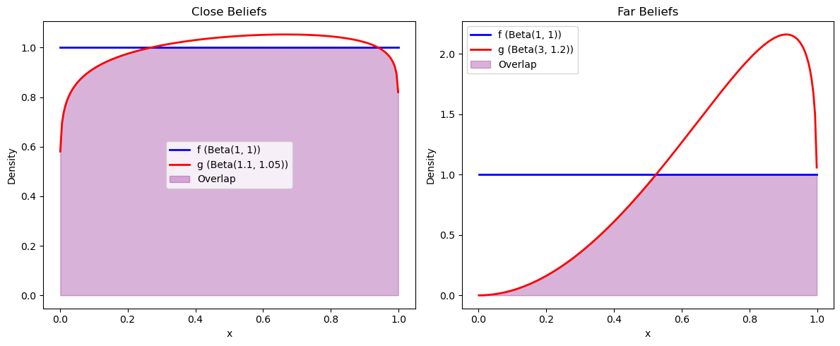
To make this idea more concrete, let’s compare two cases:
agent 1’s belief distribution \(f\) is close to agent 2’s belief distribution \(g\);
agent 1’s belief distribution \(f\) is far from agent 2’s belief distribution \(g\).
We use the two distributions visualized below
def plot_distribution_overlap(ax, x_range, f_vals, g_vals,
                            f_label='f', g_label='g',
                            f_color='blue', g_color='red'):
    """Plot two distributions with their overlap region."""
    ax.plot(x_range, f_vals, color=f_color, linewidth=2, label=f_label)
    ax.plot(x_range, g_vals, color=g_color, linewidth=2, label=g_label)

    overlap = np.minimum(f_vals, g_vals)
    ax.fill_between(x_range, 0, overlap, alpha=0.3, color='purple', label='Overlap')
    ax.set_xlabel('x')
    ax.set_ylabel('Density')
    ax.legend()

# Define close and far belief distributions
f_close = jit(lambda x: p(x, 1, 1))
g_close = jit(lambda x: p(x, 1.1, 1.05))

f_far = jit(lambda x: p(x, 1, 1))
g_far = jit(lambda x: p(x, 3, 1.2))

# Visualize the belief distributions
fig, (ax1, ax2) = plt.subplots(1, 2, figsize=(12, 5))

x_range = np.linspace(0.001, 0.999, 200)

# Close beliefs
f_close_vals = [f_close(x) for x in x_range]
g_close_vals = [g_close(x) for x in x_range]
plot_distribution_overlap(ax1, x_range, f_close_vals, g_close_vals,
                         f_label='f (Beta(1, 1))', g_label='g (Beta(1.1, 1.05))')
ax1.set_title(f'Close Beliefs')

# Far beliefs
f_far_vals = [f_far(x) for x in x_range]
g_far_vals = [g_far(x) for x in x_range]
plot_distribution_overlap(ax2, x_range, f_far_vals, g_far_vals,
                         f_label='f (Beta(1, 1))', g_label='g (Beta(3, 1.2))')
ax2.set_title(f'Far Beliefs')

plt.tight_layout()
plt.show()
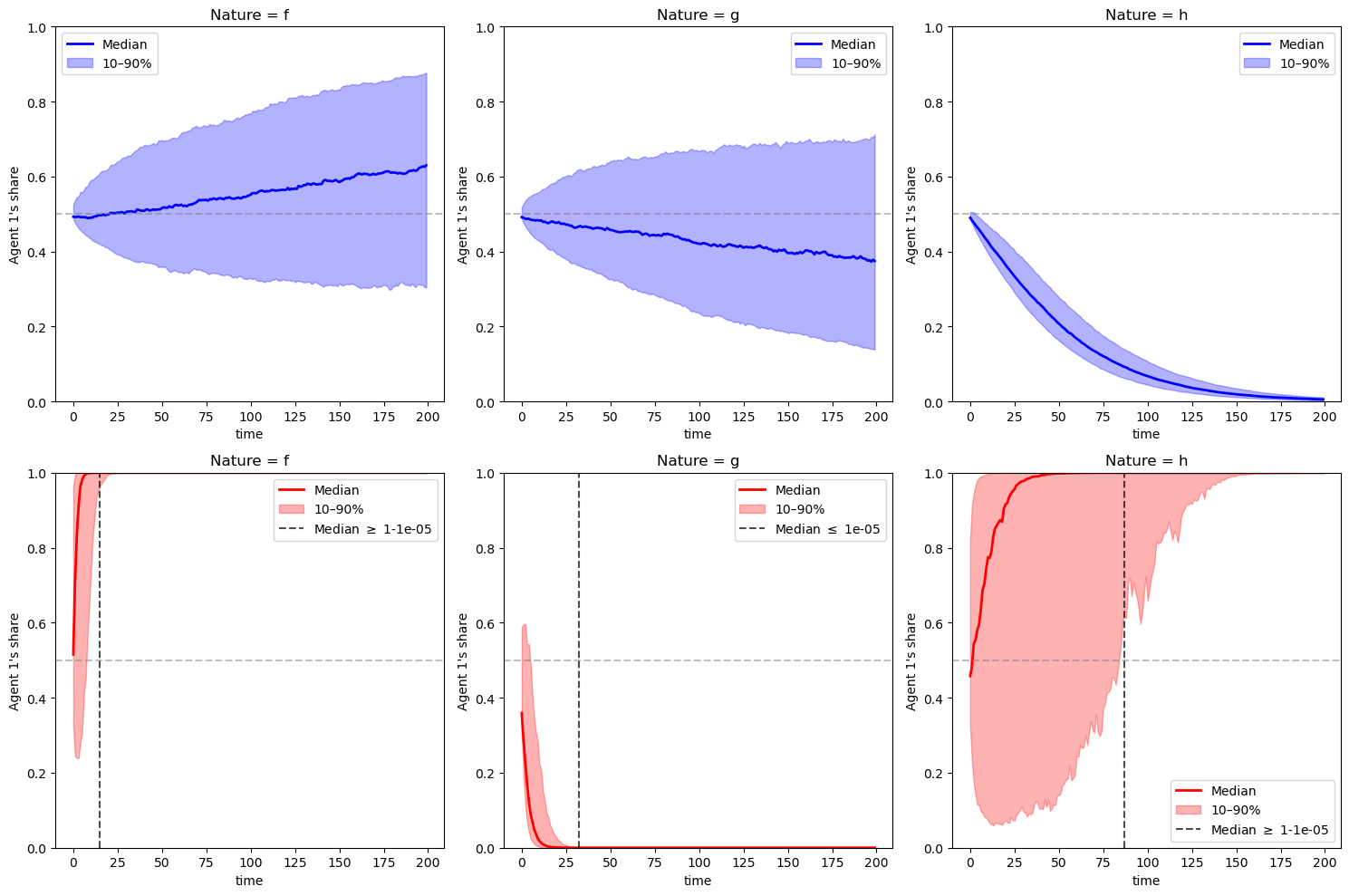
Let’s draw the same consumption ratio plots as above for agent 1.
We replace the simulation paths with median and percentiles to make the figure cleaner.
Staring at the figure below, can we infer the relation between \(KL(f,g)\) and \(KL(g,f)\)?
From the right panel, can we infer the relation between \(KL(h,g)\) and \(KL(h,f)\)?
fig, axes = plt.subplots(2, 3, figsize=(15, 10))
nature_params = {'close': [(1, 1), (1.1, 1.05), (2, 1.5)],
                 'far':   [(1, 1), (3, 1.2),   (2, 1.5)]}
nature_labels = ["Nature = f", "Nature = g", "Nature = h"]
colors = {'close': 'blue', 'far': 'red'}

threshold = 1e-5  # "close to zero" cutoff

for row, (f_belief, g_belief, label) in enumerate([
                        (f_close, g_close, 'close'),
                        (f_far, g_far, 'far')]):

    for col, nature_label in enumerate(nature_labels):
        params = nature_params[label][col]
        s_seq = np.random.beta(params[0], params[1], (1000, 200))
        _, c1 = simulate_blume_easley(s_seq, f_belief, g_belief, λ)

        median_c1 = np.median(c1, axis=0)
        p10, p90 = np.percentile(c1, [10, 90], axis=0)

        ax = axes[row, col]
        color = colors[label]
        ax.plot(median_c1, color=color, linewidth=2, label='Median')
        ax.fill_between(range(len(median_c1)), p10, p90, alpha=0.3, color=color, label='10–90%')
        ax.set_xlabel('time')
        ax.set_ylabel("Agent 1's share")
        ax.set_ylim([0, 1])
        ax.set_title(nature_label)
        ax.axhline(y=λ, color='gray', linestyle='--', alpha=0.5)
        below = np.where(median_c1 < threshold)[0]
        above = np.where(median_c1 > 1-threshold)[0]
        if below.size > 0: first_zero = (below[0], True)
        elif above.size > 0: first_zero = (above[0], False)
        else: first_zero = None
        if first_zero is not None:
            ax.axvline(x=first_zero[0], color='black', linestyle='--',
                       alpha=0.7,
                       label=fr'Median $\leq$ {threshold}' if first_zero[1]
                       else fr'Median $\geq$ 1-{threshold}')
        ax.legend()

plt.tight_layout()
plt.show()
Holding to our guesses, let’s calculate the four values
# Close case
Kf_g, Kg_f = compute_KL(f_close, g_close), compute_KL(g_close, f_close)
Kf_h, Kg_h = compute_KL_h(h, f_close, g_close)

print(f"KL divergences (close): \nKL(f,g)={Kf_g:.3f}, KL(g,f)={Kg_f:.3f}")
print(f"KL(h,f)={Kf_h:.3f}, KL(h,g)={Kg_h:.3f}")

# Far case
Kf_g, Kg_f = compute_KL(f_far, g_far), compute_KL(g_far, f_far)
Kf_h, Kg_h = compute_KL_h(h, f_far, g_far)

print(f"KL divergences (far): \nKL(f,g)={Kf_g:.3f}, KL(g,f)={Kg_f:.3f}")
print(f"KL(h,f)={Kf_h:.3f}, KL(h,g)={Kg_h:.3f}")
KL divergences (close):
KL(f,g)=0.003, KL(g,f)=0.003
KL(h,f)=0.073, KL(h,g)=0.061
KL divergences (far):
KL(f,g)=0.759, KL(g,f)=0.344
KL(h,f)=0.073, KL(h,g)=0.281
We find that in the first case, \(KL(f,g) \approx KL(g,f)\) and both are relatively small, so although either agent 1 or agent 2 will eventually consume everything, convergence displayed in the first two panels on the top is pretty slow.
In the first two panels at the bottom, we see convergence occurring faster (as indicated by the black dashed line) because the divergence gaps \(KL(f, g)\) and \(KL(g, f)\) are larger.
Since \(KL(f,g) > KL(g,f)\), we see faster convergence in the first panel at the bottom when nature chooses \(f\) than in the second panel where nature chooses \(g\).
This ties in nicely with (22.1).
23.11. Exercises#
Exercise 23.1
Starting from (23.7), show that the competitive equilibrium prices can be expressed as
Solution to Exercise 23.1
Starting from
Since both expressions equal the same price, we can equate them
Rearranging gives
where \(l_t(s^t) \equiv \pi_t^1(s^t)/\pi_t^2(s^t)\) is the likelihood ratio process.
Using \(c_t^2(s^t) = 1 - c_t^1(s^t)\):
Solving for \(c_t^1(s^t)\)
The planner’s solution gives
To match agent 1’s choice in a competitive equilibrium with the planner’s choice for agent 1, the following equality must hold
Hence we have
With \(\mu_1 = 1-\lambda\) and \(c_t^1(s^t) = \frac{\lambda l_t(s^t)}{1-\lambda+\lambda l_t(s^t)}\), we have
Since \(\pi_t^1(s^t) = l_t(s^t) \pi_t^2(s^t)\), we have
Exercise 23.2
In this exercise, we’ll study two agents, each of whom updates its posterior probability as data arrive.
each agent applies Bayes’ law in the way studied in Likelihood Ratio Processes and Bayesian Learning.
The following two models are on the table
and
as is an associated likelihood ratio process
Let \(\pi_0 \in (0,1)\) be a prior probability and
Each of our two agents deploys its own version of the mixture model
We’ll endow each type of consumer with model (23.10).
The two agents share the same \(f\) and \(g\), but
they have different initial priors, say \(\pi_0^1\) and \(\pi_0^2\)
Thus, consumer \(i\)’s probability model is
We now hand probability models (23.11) for \(i=1,2\) to the social planner.
We want to deduce allocation \(c^i(s^t), i = 1,2\), and watch what happens when
nature’s model is \(f\)
nature’s model is \(g\)
We expect that consumers will eventually learn the “truth”, but that one of them will learn faster.
To explore things, please set \(f \sim \text{Beta}(1.5, 1)\) and \(g \sim \text{Beta}(1, 1.5)\).
Please write Python code that answers the following questions.
How do consumption shares evolve?
Which agent learns faster when nature follows \(f\)?
Which agent learns faster when nature follows \(g\)?
How does a difference in initial priors \(\pi_0^1\) and \(\pi_0^2\) affect the convergence speed?
Solution to Exercise 23.2
First, let’s write helper functions that compute model components including each agent’s subjective belief function.
def bayesian_update(π_0, L_t):
    """
    Bayesian update of belief probability given likelihood ratio.
    """
    return (π_0 * L_t) / (π_0 * L_t + (1 - π_0))

def mixture_density_belief(s_seq, f_func, g_func, π_seq):
    """
    Compute the mixture density beliefs m^i(s^t) for agent i.
    """
    f_vals = f_func(s_seq)
    g_vals = g_func(s_seq)
    return π_seq * f_vals + (1 - π_seq) * g_vals
Now let’s write code that simulates the Blume-Easley model with our two agents.
def simulate_learning_blume_easley(sequences, f_belief, g_belief,
                                        π_0_1, π_0_2, λ=0.5):
    """
    Simulate Blume-Easley model with learning agents.
    """
    N, T = sequences.shape

    # Initialize arrays to store results
    π_1_seq = np.full((N, T), np.nan)
    π_2_seq = np.full((N, T), np.nan)
    c1_share = np.full((N, T), np.nan)
    l_agents_seq = np.full((N, T), np.nan)

    π_1_seq[:, 0] = π_0_1
    π_2_seq[:, 0] = π_0_2

    for n in range(N):
        # Initialize cumulative likelihood ratio for beliefs
        L_cumul = 1.0

        # Initialize likelihood ratio between agent densities
        l_agents_cumul = 1.0

        for t in range(1, T):
            s_t = sequences[n, t]

            # Compute likelihood ratio for this observation
            l_t = f_belief(s_t) / g_belief(s_t)

            # Update cumulative likelihood ratio
            L_cumul *= l_t

            # Bayesian update of beliefs
            π_1_t = bayesian_update(π_0_1, L_cumul)
            π_2_t = bayesian_update(π_0_2, L_cumul)

            # Store beliefs
            π_1_seq[n, t] = π_1_t
            π_2_seq[n, t] = π_2_t

            # Compute mixture densities for each agent
            m1_t = π_1_t * f_belief(s_t) + (1 - π_1_t) * g_belief(s_t)
            m2_t = π_2_t * f_belief(s_t) + (1 - π_2_t) * g_belief(s_t)

            # Update cumulative likelihood ratio between agents
            l_agents_cumul *= (m1_t / m2_t)
            l_agents_seq[n, t] = l_agents_cumul

            # c_t^1(s^t) = λ * l_t(s^t) / (1 - λ + λ * l_t(s^t))
            # where l_t(s^t) is the cumulative likelihood ratio between agents
            c1_share[n, t] = λ * l_agents_cumul / (1 - λ + λ * l_agents_cumul)

    return {
        'π_1': π_1_seq,
        'π_2': π_2_seq,
        'c1_share': c1_share,
        'l_agents': l_agents_seq
    }
Let’s run simulations for different scenarios.
We use \(\lambda = 0.5\), \(T=40\), and \(N=1000\).
λ = 0.5
T = 40
N = 1000

F_a, F_b = 1.5, 1
G_a, G_b = 1, 1.5

f = jit(lambda x: p(x, F_a, F_b))
g = jit(lambda x: p(x, G_a, G_b))
We’ll start with different initial priors \(\pi^i_0 \in (0, 1)\) and widen the gap between them.
# Different initial priors
π_0_scenarios = [
    (0.3, 0.7),
    (0.7, 0.3),
    (0.1, 0.9),
]
Now we can run simulations for different scenarios
# Nature follows f
s_seq_f = np.random.beta(F_a, F_b, (N, T))

# Nature follows g
s_seq_g = np.random.beta(G_a, G_b, (N, T))

results_f = {}
results_g = {}

for i, (π_0_1, π_0_2) in enumerate(π_0_scenarios):
    # When nature follows f
    results_f[i] = simulate_learning_blume_easley(
            s_seq_f, f, g, π_0_1, π_0_2, λ)
    # When nature follows g
    results_g[i] = simulate_learning_blume_easley(
            s_seq_g, f, g, π_0_1, π_0_2, λ)
Let’s visualize the results
def plot_learning_results(results, π_0_scenarios, nature_type, truth_value):
    """
    Plot beliefs and consumption shares for learning agents.
    """

    fig, axes = plt.subplots(3, 2, figsize=(10, 15))

    scenario_labels = [
        rf'$\pi_0^1 = {π_0_1}, \pi_0^2 = {π_0_2}$'
        for π_0_1, π_0_2 in π_0_scenarios
    ]

    for row, (scenario_idx, scenario_label) in enumerate(
                zip(range(3), scenario_labels)):

        res = results[scenario_idx]

        # Plot beliefs
        ax = axes[row, 0]
        π_1_med = np.median(res['π_1'], axis=0)
        π_2_med = np.median(res['π_2'], axis=0)
        ax.plot(π_1_med, 'C0', label=r'agent 1', linewidth=2)
        ax.plot(π_2_med, 'C1', label=r'agent 2', linewidth=2)
        ax.axhline(y=truth_value, color='gray', linestyle='--',
                   alpha=0.5, label=f'truth ({nature_type})')
        ax.set_title(f'Beliefs when nature = {nature_type}\n{scenario_label}')
        ax.set_ylabel(r'median $\pi_i^t$')
        ax.set_ylim([-0.05, 1.05])
        ax.legend()

        # Plot consumption shares
        ax = axes[row, 1]
        c1_med = np.median(res['c1_share'], axis=0)
        ax.plot(c1_med, 'g-', linewidth=2, label='median')
        ax.axhline(y=0.5, color='gray', linestyle='--',
                   alpha=0.5)
        ax.set_title(f'Agent 1 consumption share (Nature = {nature_type})')
        ax.set_ylabel('consumption share')
        ax.set_ylim([0, 1])
        ax.legend()

        # Add x-labels
        for col in range(2):
            axes[row, col].set_xlabel('$t$')

    plt.tight_layout()
    return fig, axes
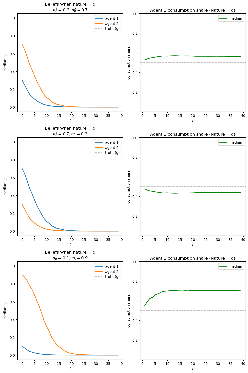
Now we’ll plot outcome when nature follows f:
fig_f, axes_f = plot_learning_results(
                results_f, π_0_scenarios, 'f', 1.0)
plt.show()
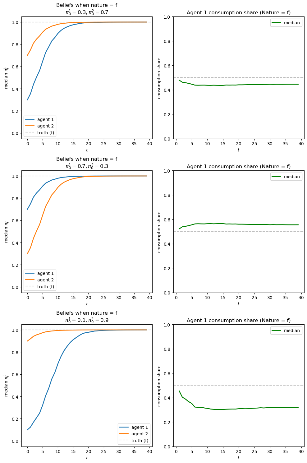
We can see that the agent with the more accurate belief gets higher consumption share.
Moreover, the further apart are initial beliefs, the longer it takes for the consumption ratio to converge.
The longer it takes for the “less accurate” agent to learn, the lower its ultimate consumption share.
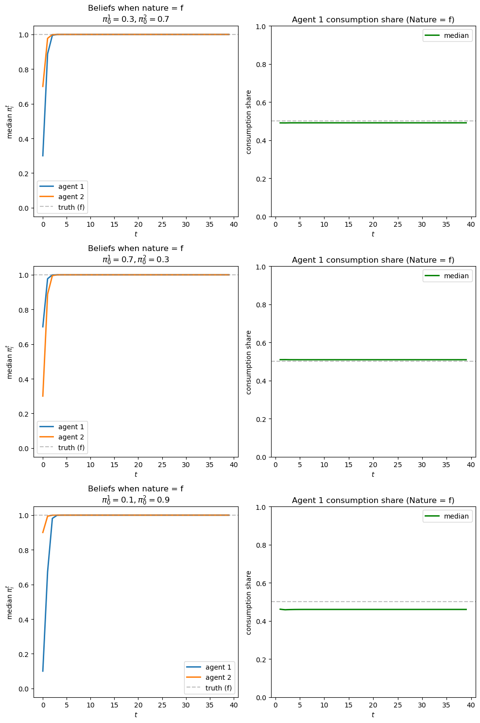
Now let’s plot outcomes when nature follows g:
fig_g, axes_g = plot_learning_results(results_g, π_0_scenarios, 'g', 0.0)
plt.show()
We observe symmetrical outcomes.
Exercise 23.3
In the previous exercise, we purposefully set the two beta distributions to be relatively close to each other.
That made it challenging to distinguish the distributions.
Now let’s study outcomes when the distributions are further apart.
Let’s set \(f \sim \text{Beta}(2, 5)\) and \(g \sim \text{Beta}(5, 2)\).
Please use the Python code you have written to study outcomes.
Solution to Exercise 23.3
Here is one solution
λ = 0.5
T = 40
N = 1000

F_a, F_b = 2, 5
G_a, G_b = 5, 2

f = jit(lambda x: p(x, F_a, F_b))
g = jit(lambda x: p(x, G_a, G_b))

π_0_scenarios = [
    (0.3, 0.7),
    (0.7, 0.3),
    (0.1, 0.9),
]

s_seq_f = np.random.beta(F_a, F_b, (N, T))
s_seq_g = np.random.beta(G_a, G_b, (N, T))

results_f = {}
results_g = {}

for i, (π_0_1, π_0_2) in enumerate(π_0_scenarios):
    # When nature follows f
    results_f[i] = simulate_learning_blume_easley(
            s_seq_f, f, g, π_0_1, π_0_2, λ)
    # When nature follows g
    results_g[i] = simulate_learning_blume_easley(
            s_seq_g, f, g, π_0_1, π_0_2, λ)
Now let’s visualize the results
fig_f, axes_f = plot_learning_results(results_f, π_0_scenarios, 'f', 1.0)
plt.show()
fig_g, axes_g = plot_learning_results(results_g, π_0_scenarios, 'g', 0.0)
plt.show()
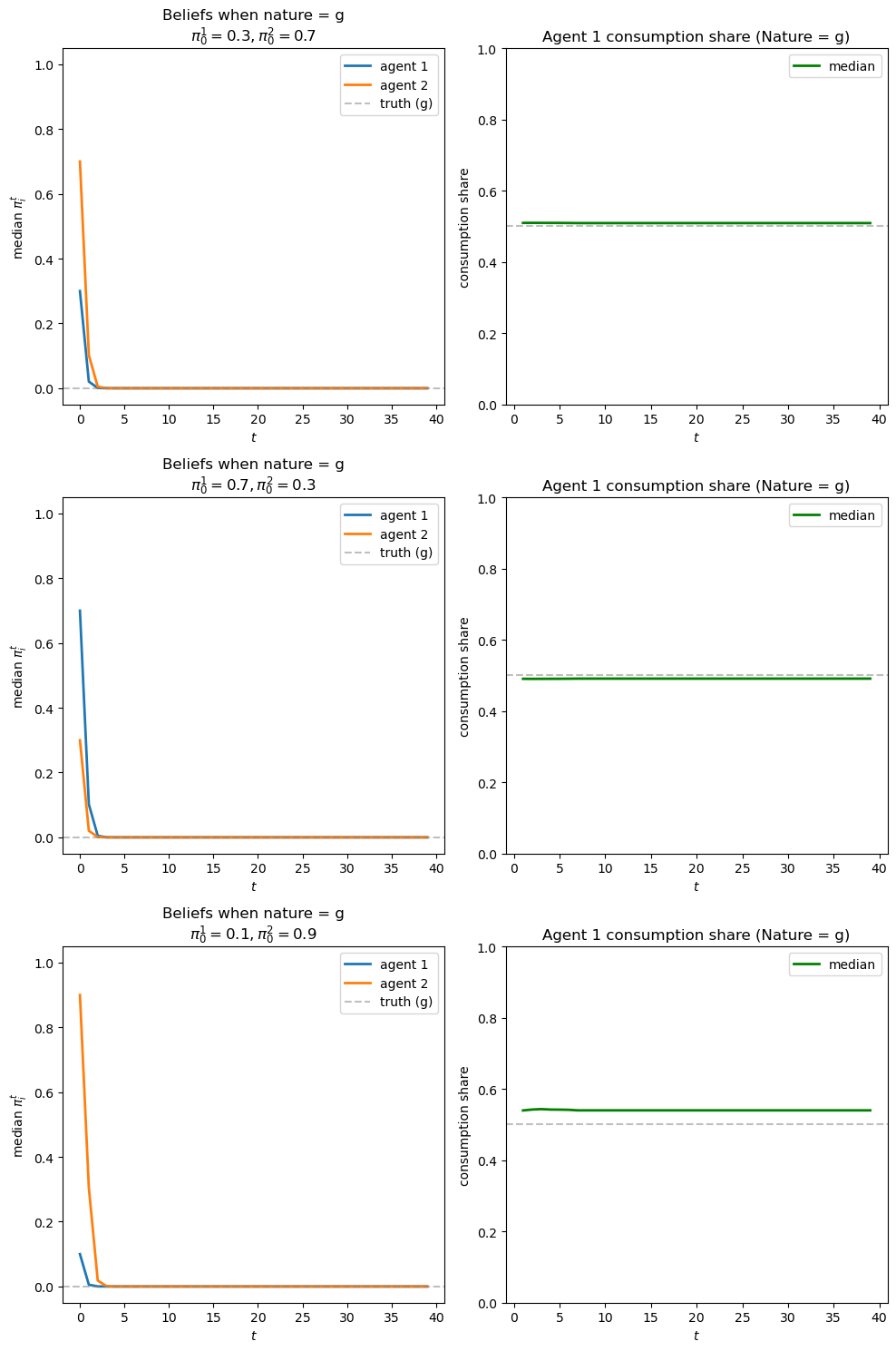
Evidently, because the two distributions are further apart, it is easier to distinguish them.
So learning occurs more quickly.
So do consumption shares.
Exercise 23.4
Two agents have different beliefs about three possible models.
Assume \(f(x) \geq 0\), \(g(x) \geq 0\), and \(h(x) \geq 0\) for \(x \in X\) with:
\(\int_X f(x) dx = 1\)
\(\int_X g(x) dx = 1\)
\(\int_X h(x) dx = 1\)
We’ll consider two agents:
Agent 1: \(\pi^g_0 = 1 - \pi^f_0\), \(\pi^f_0 \in (0,1), \pi^h_0 = 0\) (attaches positive probability only to models \(f\) and \(g\))
Agent 2: \(\pi^g_0 = \pi^f_0 = 1/3\), \(\pi^h_0 = 1/3\) (attaches equal weights to all three models)
Let \(f\) and \(g\) be two beta distributions with \(f \sim \text{Beta}(3, 2)\) and \(g \sim \text{Beta}(2, 3)\), and set \(h = \pi^f_0 f + (1-\pi^f_0) g\) with \(\pi^f_0 = 0.5\).
Bayes’ Law tells us that posterior probabilities on models \(f\) and \(g\) evolve according to
and
Please simulate and visualize evolutions of posterior probabilities and consumption allocations when:
Nature permanently draws from \(f\)
Nature permanently draws from \(g\)
Solution to Exercise 23.4
Let’s implement this three-model case with two agents having different beliefs.
Let’s define \(f\) and \(g\) far apart, with \(h\) being a mixture of \(f\) and \(g\).
F_a, F_b = 3, 2
G_a, G_b = 2, 3
λ = 0.5
π_f_0 = 0.5

f = jit(lambda x: p(x, F_a, F_b))
g = jit(lambda x: p(x, G_a, G_b))
h = jit(lambda x: π_f_0 * f(x) + (1 - π_f_0) * g(x))
Now we can define the belief updating for the model
@jit(parallel=True)
def compute_posterior_three_models(
    s_seq, f_func, g_func, h_func, π_f_0, π_g_0):
    """
    Compute posterior probabilities for three models.
    """
    N, T = s_seq.shape
    π_h_0 = 1 - π_f_0 - π_g_0

    π_f = np.zeros((N, T))
    π_g = np.zeros((N, T))
    π_h = np.zeros((N, T))

    for n in prange(N):
        # Initialize with priors
        π_f[n, 0] = π_f_0
        π_g[n, 0] = π_g_0
        π_h[n, 0] = π_h_0

        # Compute cumulative likelihoods
        f_cumul = 1.0
        g_cumul = 1.0
        h_cumul = 1.0

        for t in range(1, T):
            s_t = s_seq[n, t]

            # Update cumulative likelihoods
            f_cumul *= f_func(s_t)
            g_cumul *= g_func(s_t)
            h_cumul *= h_func(s_t)

            # Compute posteriors using Bayes' rule
            denominator = π_f_0 * f_cumul + π_g_0 * g_cumul + π_h_0 * h_cumul

            π_f[n, t] = π_f_0 * f_cumul / denominator
            π_g[n, t] = π_g_0 * g_cumul / denominator
            π_h[n, t] = π_h_0 * h_cumul / denominator

    return π_f, π_g, π_h
Let’s also write simulation code along the lines of earlier exercises
@jit
def bayesian_update_three_models(π_f_0, π_g_0, L_f, L_g, L_h):
    """Bayesian update for three models."""
    π_h_0 = 1 - π_f_0 - π_g_0
    denom = π_f_0 * L_f + π_g_0 * L_g + π_h_0 * L_h
    return π_f_0 * L_f / denom, π_g_0 * L_g / denom, π_h_0 * L_h / denom

@jit
def compute_mixture_density(π_f, π_g, π_h, f_val, g_val, h_val):
    """Compute mixture density for an agent."""
    return π_f * f_val + π_g * g_val + π_h * h_val

@jit(parallel=True)
def simulate_three_model_allocation(sequences, f_func, g_func, h_func,
                                     π_f_0_1, π_g_0_1, π_f_0_2, π_g_0_2, λ=0.5):
    """
    Simulate Blume-Easley model with learning agents and three models.
    """
    N, T = sequences.shape

    # Initialize arrays to store results
    beliefs_1 = {k: np.full((N, T), np.nan) for k in ['π_f', 'π_g', 'π_h']}
    beliefs_2 = {k: np.full((N, T), np.nan) for k in ['π_f', 'π_g', 'π_h']}
    c1_share = np.full((N, T), np.nan)
    l_agents_seq = np.full((N, T), np.nan)

    # Set initial beliefs
    beliefs_1['π_f'][:, 0] = π_f_0_1
    beliefs_1['π_g'][:, 0] = π_g_0_1
    beliefs_1['π_h'][:, 0] = 1 - π_f_0_1 - π_g_0_1
    beliefs_2['π_f'][:, 0] = π_f_0_2
    beliefs_2['π_g'][:, 0] = π_g_0_2
    beliefs_2['π_h'][:, 0] = 1 - π_f_0_2 - π_g_0_2

    for n in range(N):
        # Initialize cumulative likelihoods
        L_cumul = {'f': 1.0, 'g': 1.0, 'h': 1.0}
        l_agents_cumul = 1.0

        # Calculate initial consumption share at t=0
        l_agents_seq[n, 0] = 1.0
        c1_share[n, 0] = λ * 1.0 / (1 - λ + λ * 1.0)  # This equals λ

        for t in range(1, T):
            s_t = sequences[n, t]

            # Compute densities for current observation
            densities = {
                'f': f_func(s_t),
                'g': g_func(s_t),
                'h': h_func(s_t)
            }

            # Update cumulative likelihoods
            for model in L_cumul:
                L_cumul[model] *= densities[model]

            # Bayesian updates for both agents
            π_f_1, π_g_1, π_h_1 = bayesian_update_three_models(
                π_f_0_1, π_g_0_1, L_cumul['f'], L_cumul['g'], L_cumul['h'])
            π_f_2, π_g_2, π_h_2 = bayesian_update_three_models(
                π_f_0_2, π_g_0_2, L_cumul['f'], L_cumul['g'], L_cumul['h'])

            # Store beliefs
            beliefs_1['π_f'][n, t] = π_f_1
            beliefs_1['π_g'][n, t] = π_g_1
            beliefs_1['π_h'][n, t] = π_h_1
            beliefs_2['π_f'][n, t] = π_f_2
            beliefs_2['π_g'][n, t] = π_g_2
            beliefs_2['π_h'][n, t] = π_h_2

            # Compute mixture densities
            m1_t = compute_mixture_density(
                π_f_1, π_g_1, π_h_1, densities['f'],
                densities['g'], densities['h'])
            m2_t = compute_mixture_density(
                π_f_2, π_g_2, π_h_2, densities['f'],
                densities['g'], densities['h'])

            # Update cumulative likelihood ratio between agents
            l_agents_cumul *= (m1_t / m2_t)
            l_agents_seq[n, t] = l_agents_cumul

            # Consumption share for agent 1
            c1_share[n, t] = λ * l_agents_cumul / (1 - λ + λ * l_agents_cumul)

    return {
        'π_f_1': beliefs_1['π_f'],
        'π_g_1': beliefs_1['π_g'],
        'π_h_1': beliefs_1['π_h'],
        'π_f_2': beliefs_2['π_f'],
        'π_g_2': beliefs_2['π_g'],
        'π_h_2': beliefs_2['π_h'],
        'c1_share': c1_share,
        'l_agents': l_agents_seq
    }
The following code cell defines a plotting function to show evolutions of beliefs and consumption ratios
Now let’s run the simulation.
In the simulation below, agent 1 assigns positive probabilities only to \(f\) and \(g\), while agent 2 puts equal weights on all three models.
T = 100
N = 1000

# Generate sequences for nature f and g
s_seq_f = np.random.beta(F_a, F_b, (N, T))
s_seq_g = np.random.beta(G_a, G_b, (N, T))

# Run simulations
results_f = simulate_three_model_allocation(s_seq_f,
                        f, g, h, π_f_0, 1-π_f_0,
                        1/3, 1/3, λ)
results_g = simulate_three_model_allocation(s_seq_g,
                        f, g, h, π_f_0, 1-π_f_0,
                        1/3, 1/3, λ)
Plots below show the evolution of beliefs for each model (f, g, h) separately.
First we show the figure when nature chooses \(f\)
plot_belief_evolution(results_f, nature='f', figsize=(15, 5))
plt.show()
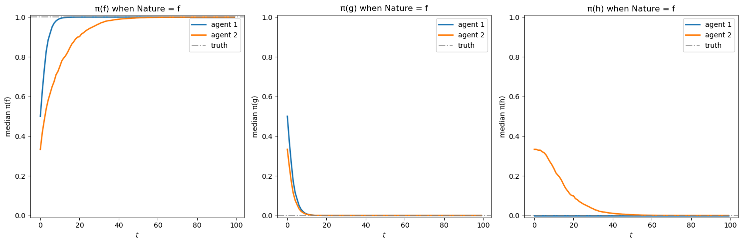
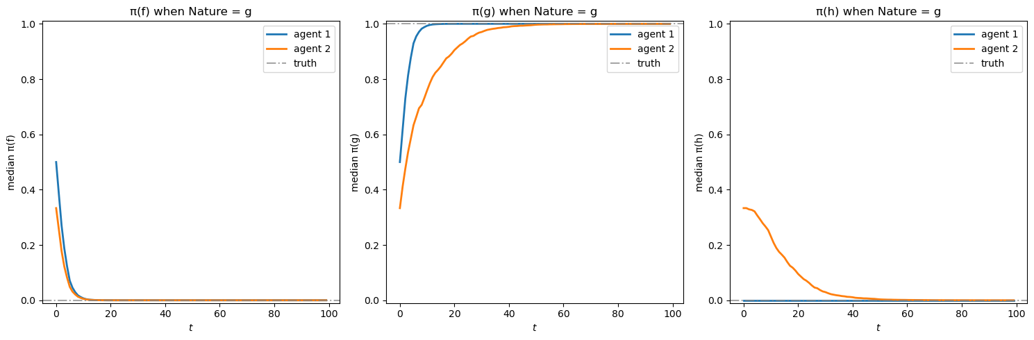
Agent 1’s posterior beliefs are depicted in blue and agent 2’s posterior beliefs are depicted in orange.
Evidently, when nature draws from \(f\), agent 1 learns faster than agent 2, who, unlike agent 1, attaches a positive prior probability to model \(h\):
In the leftmost panel, both agents’ beliefs for \(\pi(f)\) converge toward 1 (the truth)
Agent 2’s belief in model \(h\) (rightmost panel) gradually converges to 0 after an initial rise
Now let’s plot the belief evolution when nature chooses \(g\):
plot_belief_evolution(results_g, nature='g', figsize=(15, 5))
plt.show()
Again, agent 1 learns faster than agent 2.
Before reading the next figure, please guess how consumption shares evolve.
Remember that agent 1 reaches the correct model faster than agent 2
plot_consumption_dynamics(results_f, results_g, λ=0.5, figsize=(14, 5))
plt.show()
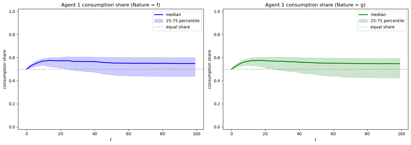
As we expected, agent 1 has a higher consumption share compared to agent 2.
In this exercise, the “truth” is among possible outcomes according to both agents.
Agent 2’s model is “more general” because it allows a possibility – that nature is drawing from \(h\) – that agent 1’s model does not include.
Agent 1 learns more quickly because he uses a simpler model.
Exercise 23.5
Now consider two agents with extreme priors about three models.
Consider the same setup as the previous exercise, but now:
Agent 1: \(\pi^g_0 = \pi^f_0 = \frac{\epsilon}{2} > 0\), where \(\epsilon\) is close to \(0\) (e.g., \(\epsilon = 0.01\))
Agent 2: \(\pi^g_0 = \pi^f_0 = 0\) (rigid belief in model \(h\))
Choose \(h\) to be close but not equal to either \(f\) or \(g\) as measured by KL divergence. For example, set \(h \sim \text{Beta}(1.2, 1.1)\) and \(f \sim \text{Beta}(1, 1)\).
Please simulate and visualize evolutions of posterior probabilities and consumption allocations when:
Nature permanently draws from \(f\)
Nature permanently draws from \(g\)
Solution to Exercise 23.5
To explore this exercise, we increase \(T\) to 1000.
Let’s specify \(f, g\), and \(h\) and verify that \(h\) and \(f\) are closer than \(h\) and \(g\)
F_a, F_b = 1, 1
G_a, G_b = 3, 1.2
H_a, H_b = 1.2, 1.1

f = jit(lambda x: p(x, F_a, F_b))
g = jit(lambda x: p(x, G_a, G_b))
h = jit(lambda x: p(x, H_a, H_b))

Kh_f = compute_KL(h, f)
Kh_g = compute_KL(h, g)
Kf_h = compute_KL(f, h)
Kg_h = compute_KL(g, h)

print(f"KL divergences:")
print(f"KL(h,f) = {Kh_f:.4f}, KL(h,g) = {Kh_g:.4f}")
print(f"KL(f,h) = {Kf_h:.4f}, KL(g,h) = {Kg_h:.4f}")
KL divergences:
KL(h,f) = 0.0092, KL(h,g) = 0.5514
KL(f,h) = 0.0105, KL(g,h) = 0.2919
Now we can set the belief models for the two agents
ε = 0.01
λ = 0.5

# Agent 1: π_f = ε/2, π_g = ε/2, π_h = 1-ε
# (almost rigid about h)
π_f_1 = ε/2
π_g_1 = ε/2

# Agent 2: π_f = 0, π_g = 0, π_h = 1
# (fully rigid about h)
π_f_2 = 1e-10
π_g_2 = 1e-10
Now we can run the simulation
T = 1000
N = 1000

# Generate sequences for different nature scenarios
s_seq_f = np.random.beta(F_a, F_b, (N, T))
s_seq_g = np.random.beta(G_a, G_b, (N, T))

# Run simulations for both scenarios
results_f = simulate_three_model_allocation(
                                s_seq_f,
                                f, g, h,
                                π_f_1, π_g_1, π_f_2, π_g_2, λ)
results_g = simulate_three_model_allocation(
                                s_seq_g,
                                f, g, h,
                                π_f_1, π_g_1, π_f_2, π_g_2, λ)
Let’s plot the belief evolution when nature chooses \(f\)
plot_belief_evolution(results_f, nature='f', figsize=(15, 5))
plt.show()
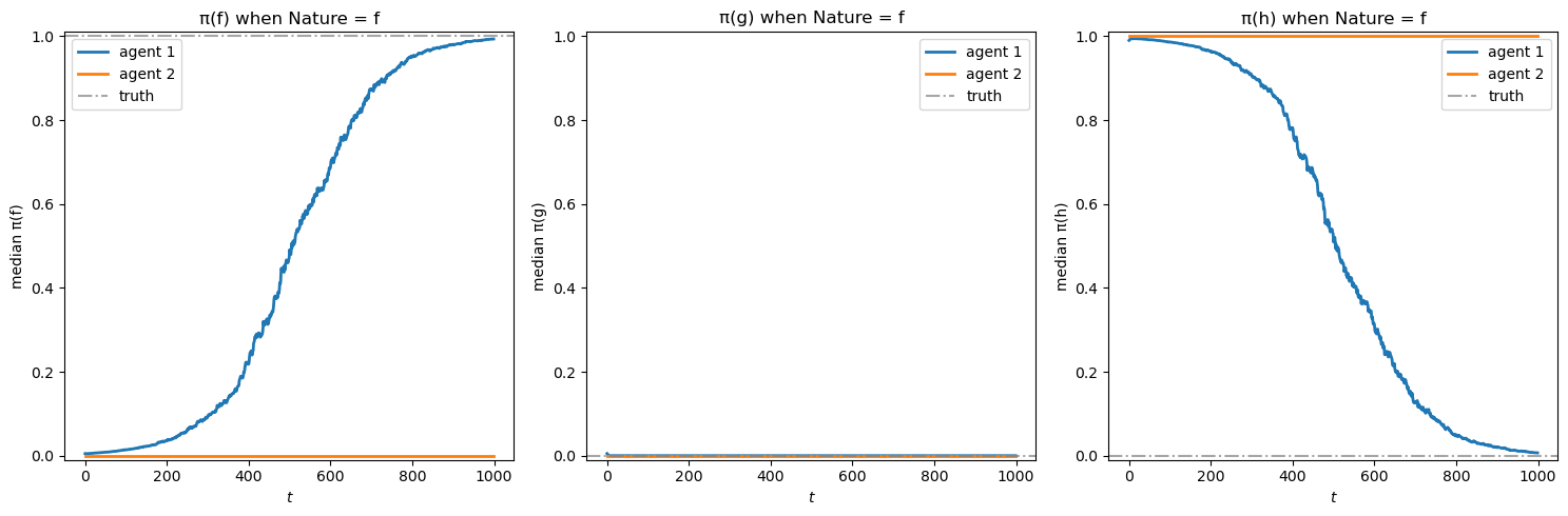
Observe how slowly agent 1 learns the truth in the leftmost panel showing \(\pi(f)\).
Also note that agent 2 is not updating.
This is because we have specified that \(f\) is very difficult to distinguish from \(h\) as measured by \(KL(f, h)\).
The rigidity regarding \(h\) prevents agent 2 from updating its beliefs when observing a very similar model \(f\)
Now let’s plot the belief evolution when nature chooses \(g\)
plot_belief_evolution(results_g, nature='g', figsize=(15, 5))
plt.show()
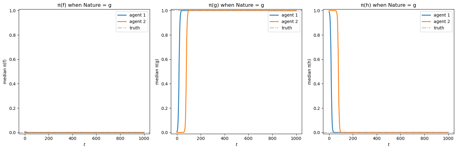
When nature draws from \(g\), it is further away from \(h\) as measured by the KL divergence.
This helps both agents learn the truth more quickly.
plot_consumption_dynamics(results_f, results_g,
                               λ=0.5, figsize=(14, 5))
plt.show()
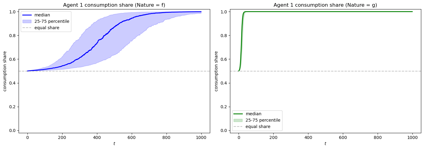
In the consumption dynamics plot, notice that agent 1’s consumption share converges to 1 both when nature permanently draws from \(f\) and when nature permanently draws from \(g\).
23.6. Social planner’s allocation problem#
The benevolent dictator has all the information it requires to choose a consumption allocation that maximizes the social welfare criterion
where \(\lambda \in [0,1]\) is a Pareto weight that tells how much the planner likes agent \(1\) and \(1 - \lambda\) is a Pareto weight that tells how much the social planner likes agent \(2\).
Setting \(\lambda = .5\) expresses ‘‘egalitarian’’ social preferences.
Notice how social welfare criterion (23.3) takes into account both agents’ preferences as represented by formula (23.2).
This means that the social planner knows and respects
each agent’s one period utility function \(u(\cdot) = \ln(\cdot)\)
each agent \(i\)’s probability model \(\{\pi_t^i(s^t)\}_{t=0}^\infty\)
Consequently, we anticipate that these objects will appear in the social planner’s rule for allocating the aggregate endowment each period.
First-order necessary conditions for maximizing welfare criterion (23.3) subject to the feasibility constraint (23.1) are
which can be rearranged to become
where
is the likelihood ratio of agent 1’s joint density to agent 2’s joint density.
Using
we can rewrite allocation rule (23.4) as
or
which implies that the social planner’s allocation rule is
If we define a temporary or continuation Pareto weight process as
then we can represent the social planner’s allocation rule as